
Introduction to Modulation Transfer Function
When optical designers attempt to compare the performance of optical systems, a commonly used measure is the modulation transfer function (MTF). MTF is used for components as simple as a spherical singlet lens to those as complex as a multi-element ecentric imaging lens assembly. In order to understand the significance of MTF, consider some general principles and practical examples for defining MTF including its components, importance, and characterization.
THE COMPONENTS OF MTF
To properly define the modulation transfer function, it is necessary to first define two terms required to truly characterize image performance: resolution and contrast.
Resolution
Resolution is an imaging system's ability to distinguish object detail. It is often expressed in terms of line-pairs per millimeter (where a line-pair is a sequence of one black line and one white line). This measure of line-pairs per millimeter (lp/mm) is also known as frequency. The inverse of the frequency yields the spacing in millimeters between two resolved lines. Bar targets with a series of equally spaced, alternating white and black bars (i.e. a 1951 USAF target or a Ronchi ruling) are ideal for testing system performance. For a more detailed explanation of test targets, view Choosing the Correct Test Target. For all imaging optics, when imaging such a pattern, perfect line edges become blurred to a degree (Figure 1). High-resolution images are those which exhibit a large amount of detail as a result of minimal blurring. Conversely, low-resolution images lack fine detail.
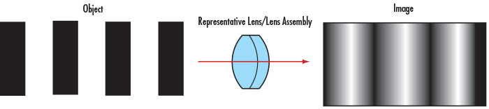
Figure 1: Perfect Line Edges Before (Left) and After (Right) Passing through a Low Resolution Imaging Lens
A practical way of understanding line-pairs is to think of them as pixels on a camera sensor, where a single line-pair corresponds to two pixels (Figure 2). Two camera sensor pixels are needed for each line-pair of resolution: one pixel is dedicated to the red line and the other to the blank space between pixels. Using the aforementioned metaphor, image resolution of the camera can now be specified as equal to twice its pixel size.
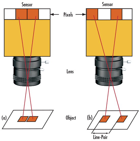
Figure 2: Imaging Scenarios Where (a) the Line-Pair is NOT Resolved and (b) the Line-Pair is Resolved
Correspondingly, object resolution is calculated using the camera resolution and the primary magnification (PMAG) of the imaging lens (Equations 1 – 2). It is important to note that these equations assume the imaging lens contributes no resolution loss.


Contrast/Modulation
Consider normalizing the intensity of a bar target by assigning a maximum value to the white bars and zero value to the black bars. Plotting these values results in a square wave, from which the notion of contrast can be more easily seen (Figure 3). Mathematically, contrast is calculated with Equation 3:

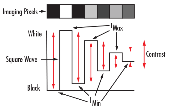
Figure 3: Contrast Expressed as a Square Wave
When this same principle is applied to the imaging example in Figure 1, the intensity pattern before and after imaging can be seen (Figure 4). Contrast or modulation can then be defined as how faithfully the minimum and maximum intensity values are transferred from object plane to image plane.
To understand the relation between contrast and image quality, consider an imaging lens with the same resolution as the one in Figure 1 and Figure 4, but used to image an object with a greater line-pair frequency. Figure 5 illustrates that as the spatial frequency of the lines increases, the contrast of the image decreases. This effect is always present when working with imaging lenses of the same resolution. For the image to appear defined, black must be truly black and white truly white, with a minimal amount of grayscale between.
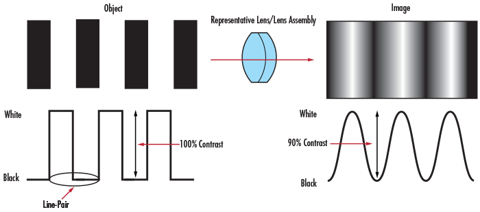
Figure 4: Contrast of a Bar Target and Its Image
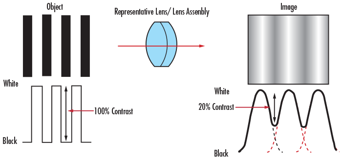
Figure 5: Contrast Comparison at Object and Image Planes
In imaging applications, the imaging lens, camera sensor, and illumination play key roles in determining the resulting image contrast. The lens contrast is typically defined in terms of the percentage of the object contrast that is reproduced. The sensor's ability to reproduce contrast is usually specified in terms of decibels (dB) in analog cameras and bits in digital cameras.
UNDERSTANDING MTF
Now that the components of the modulation transfer function (MTF), resolution and contrast/modulation, are defined, consider MTF itself. The MTF of a lens, as the name implies, is a measurement of its ability to transfer contrast at a particular resolution from the object to the image. In other words, MTF is a way to incorporate resolution and contrast into a single specification. As line spacing decreases (i.e. the frequency increases) on the test target, it becomes increasingly difficult for the lens to efficiently transfer this decrease in contrast; as result, MTF decreases (Figure 6).
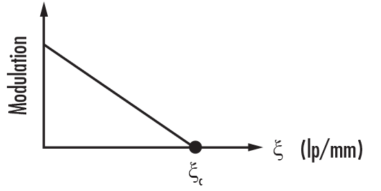
Figure 6: MTF for an Aberration-Free Lens with a Rectangular Aperture
For an aberration-free image with a circular pupil, MTF is given by Equation 4, where MTF is a function of spatial resolution (ξ), which refers to the smallest line-pair the system can resolve. The cut-off frequency (ξc) is given by Equation 6.
Figure 6 plots the MTF of an aberration-free image with a rectangular pupil. As can be expected, the MTF decreases as the spatial resolution increases. It is important to note that these cases are idealized and that no actual system is compley aberration-free.



THE IMPORTANCE OF MTF
In traditional system integration (and less crucial applications), the system's performance is roughly estimated using the principle of the weakest link. The principle of the weakest link proposes that a system's resolution is solely limited by the component with the lowest resolution. Although this approach is very useful for quick estimations, it is actually flawed because every component within the system contributes error to the image, yielding poorer image quality than the weakest link alone.
Every component within a system has an associated modulation transfer function (MTF) and, as a result, contributes to the overall MTF of the system. This includes the imaging lens, camera sensor, image capture boards, and video cables, for instance. The resulting MTF of the system is the product of all the MTF curves of its components (Figure 7). For instance, a 25mm fixed focal length lens and a 25mm double gauss lens can be compared by evaluating the resulting system performance of both lenses with a Sony monochrome camera. By analyzing the system MTF curve, it is straightforward to determine which combination will yield sufficient performance. In some metrology applications, for example, a certain amount of contrast is required for accurate image edge detection. If the minimum contrast needs to be 35% and the image resolution required is 30 lp/mm, then the 25mm double gauss lens is the best choice.
MTF is one of the best tools available to quantify the overall imaging performance of a system in terms of resolution and contrast. As a result, knowing the MTF curves of each imaging lens and camera sensor within a system allows a designer to make the appropriate selection when optimizing for a particular resolution.
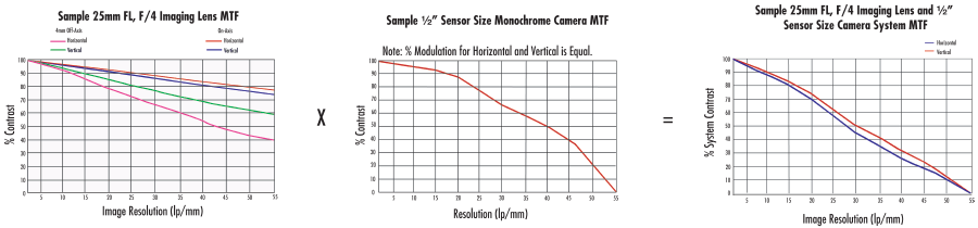
Figure 7: System MTF is the Product of the MTF of Individual Component: Lens MTF x Camera MTF = System MTF
CHARACTERIZATION OF MTF
Determining Real-World MTF
A theoretical modulation transfer function (MTF) curve can be generated from the optical prescription of any lens. Although this can be helpful, it does not indicate the actual, real-world performance of the lens after accounting for manufacturing tolerances. Manufacturing tolerances always introduce some performance loss to the original optical design since factors such as geometry and coating deviate slightly from an ideal lens or lens system. For this reason, in our manufacturing sites, Edmund Optics® invests in optical test and measurement equipment for quantifying MTF. This MTF test and measurement equipment allows for characterization of the actual performance of both designed lenses and commercial lenses (whose optical prescription is not available to the public). As a result, precise integration - previously limited to lenses with known prescriptions - can now include commercial lenses.
Reading MTF Graphs/Data
Reading Modulation Transfer Function Graphs/Data
A greater area under the MTF curve does not always indicate the optimal choice. A designer should decide based on the resolution of the application at hand. As previously discussed, an MTF graph plots the percentage of transferred contrast versus the frequency (cycles/mm) of the lines. A few things should be noted about the MTF curves offered by Edmund Optics®:
Each MTF curve is calculated for a single point in space. Typical field points include on-axis, 70% field, and full-field. 70% is a common reference point because it captures approximay 50% of the total imaging area.
Off-axis MTF data is calculated for both tangential and sagittal cases (denoted by T and S, respectively). Occasionally an average of the two is presented rather than the two individual curves.
MTF curves are dependent on several factors, such as system conjugates, wavebands, and f/#. An MTF curve is calculated at specified values of each; therefore, it is important to review these factors before determining whether a component will work for a certain application.
The spatial frequency is expressed in terms of cycles (or line-pairs) per millimeter. The inverse of this frequency yields the spacing of a line-pair (a cycle of one black bar and one white bar) in millimeters.
The nominal MTF curve is generated using the standard prescription information available in optical design programs. This prescription information can also be found on our global website, in our print catalogs, and in our lens catalogs supplied to Zemax®. The nominal MTF represents the best-case scenario and does not take into account manufacturing tolerances.
Conceptually, MTF can be difficult to grasp. Perhaps the easiest way to understand this notion of transferring contrast from object to image plane is by examining a real-world example. Figures 8 - 12 compare MTF curves and images for two 25mm fixed focal length imaging lenses: #54-855 Finite Conjugate Micro-Video Lens and #59-871 Compact Fixed Focal Length Lens. Figure 8 shows polychromatic diffraction MTF for these two lenses. Depending upon the testing conditions, both lenses can yield equivalent performance. In this particular example, both are trying to resolve group 2, elements 5 -6 (indicated by the red boxes in Figure 10) and group 3, elements 5 – 6 (indicated by the blue boxes in Figure 10) on a 1951 USAF resolution target (Figure 9). In terms of actual object size, group 3, elements 5 – 6 represent 6.35 – 7.13lp/mm (14.03 - 15.75μm) and group 3, elements 5 – 6 represent 12.70 – 14.25lp/mm (7.02 - 7.87μm). For an easy way to calculate resolution given element and group numbers, use our 1951 USAF Resolution EO Tech Tool.
Under the same testing parameters, it is clear to see that #59-871 (with a better MTF curve) yields better imaging performance compared to #54-855 (Figures 11 – 12). In this real-world example with these particular 1951 USAF elements, a higher modulation value at higher spatial frequencies corresponds to a clearer image; however, this is not always the case. Some lenses are designed to be able to very accuray resolve lower spatial frequencies, and have a very low cut-off frequency (i.e. they cannot resolve higher spatial frequencies). Had the target been group -1, elements 5-6, the two lenses would have produced much more similar images given their modulation values at lower frequencies.
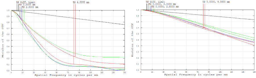
Figure 8: Comparison of Polychromatic Diffraction MTF for #54-855 Finite Conjugate Micro-Video Lens (Left) and #59-871 Compact Fixed Focal Length Lens (Right)

Figure 9: 1951 USAF Resolution Target

Figure 10: Comparison of #54-855 Finite Conjugate Micro-Video Lens (Left) and #59-871 Compact Fixed Focal Length Lens (Right) Resolving Group 2, Elements 5 -6 (Red Boxes) and Group 3, Elements 5 – 6 (Blue Boxes) on a 1951 USAF Resolution Target
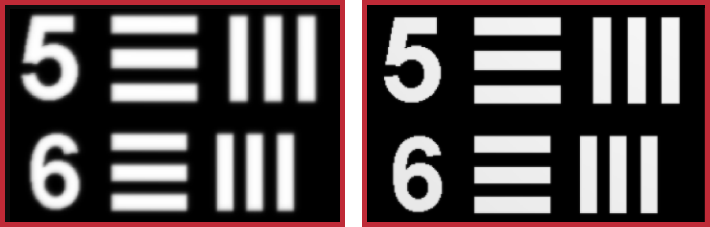
Figure 11: Comparison of #54-855 Finite Conjugate Micro-Video Lens (Left) and #59-871 Compact Fixed Focal Length Lens (Right) Resolving Group 2, Elements 5 -6 on a 1951 USAF Resolution Target

Figure 12: Comparison of #54-855 Finite Conjugate Micro-Video Lens (Left) and #59-871 Compact Fixed Focal Length Lens (Right) Resolving Group 3, Elements 5 – 6 on a 1951 USAF Resolution Target
Modulation transfer function (MTF) is one of the most important parameters by which image quality is measured. Optical designers and engineers frequently refer to MTF data, especially in applications where success or failure is contingent on how accuray a particular object is imaged. To truly grasp MTF, it is necessary to first understand the ideas of resolution and contrast, as well as how an object's image is transferred from object to image plane. While initially daunting, understanding and eventually interpreting MTF data is a very powerful tool for any optical designer. With knowledge and experience, MTF can make selecting the appropriate lens a far easier endeavor - despite the multitude of offerings.
版權所有 © 2026 江陰韻翔光電技術有限公司 備案號:蘇ICP備16003332號-1 技術支持:化工儀器網 管理登陸 GoogleSitemap


